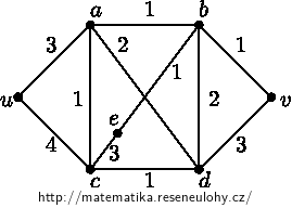
We fill in the table, where for individual vertices we present an estimate \( d \) of the distance from \( u \), the just processed vertex \( x \) and the set of already processed vertices \( Z \). The line indicates the values \( d, x \) and \( Z \) after performing the appropriate iteration.
\(
\begin{array}{c|ccccccc|c|l}
\# & u & a & b & c & d & e & v & x & Z \\
0 & 0 & \infty & \infty & \infty & \infty & \infty & \infty & & \emptyset \\
1 & 0 & 3 & \infty & 4 & \infty & \infty & \infty & u & u \\
2 & 0 & 3 & 5 & 4 & 5 & \infty & \infty & a & u,a \\
3 & 0 & 3 & 5 & 4 & 5 & 7 & \infty & c & u,a,c \\
4 & 0 & 3 & 5 & 4 & 5 & 7 & 8 & d & u,a,c,d \\
5 & 0 & 3 & 5 & 4 & 5 & 7 & 6 & b & u,a,c,d,b \\
6 & 0 & 3 & 5 & 4 & 5 & 6 & 6 & v & u,a,c,d,b, v \\
\end{array}
\)
Note that the execution of the algorithm is not unique. In the fourth iteration, we chose \( x \) between \( d \) and \( b \). Similarly, in the last iteration, \( e \) could be chosen instead of \( in \). The algorithm would then have one more iteration.
Not all vertices were processed. At the end of the algorithm \( e \notin Z \).
")


